Installation Guide

1. These instructions are for Ubuntu 22.04 LTS either natively or running in WSL2.
2. Download the MMWAVE-L-SDK for xWRL6432 from https://www.ti.com/tool/MMWAVE-L-SDK. Install it in C:/ti on Windows or ~/ti on Ubuntu.
3. Download SysConfig from https://www.ti.com/tool/SYSCONFIG. Install it in C:/ti on Windows or ~/ti on Ubuntu.
4. Download the TI CLANG Compiler Toolchain from https://www.ti.com/tool/TI-CLANG. Install it in C:/ti on Windows or ~/ti on Ubuntu.
5. Download and install Python 3.10 from https://www.python.org/downloads/. Make sure to add it to your path.
6. Make sure the Python package manager pip is installed.
7. Install the packages needed for the flashing tools with pip install pyserial xmodem tqdm.
8. If on Ubuntu, install mono runtime with sudo apt install mono-runtime.
9. Download Code Composer Studio (CCS) from https://www.ti.com/tool/CCSTUDIO.
10. Install CCS by running the installer file after unzipping the package.
    • Keep the default installation path.
    • Select the component “mmwave” to install xWRL6432 support.
    • Launch CCS with the default workspace.
    • Go to Window > Preferences > Code Composer Studio > Products and make sure SysConfig is listed.
    • Go to Window > Preferences > Code Composer Studio > Build > Compilers and make sure TI Clang is listed.

Getting To Know the Hardware

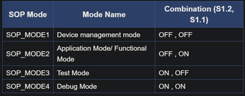
The board has 4 different modes controlled by the switches on the board:

Flashing Process

(Recommended to perform the following steps on a Windows filesystem)

1. Download flashing tool from UniFlash.
2. Connect the mmWave radar to your computer.

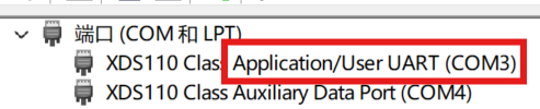
3. Check which port is being used by looking at the Device Manager; we need the Application UART (COM3 in this case)

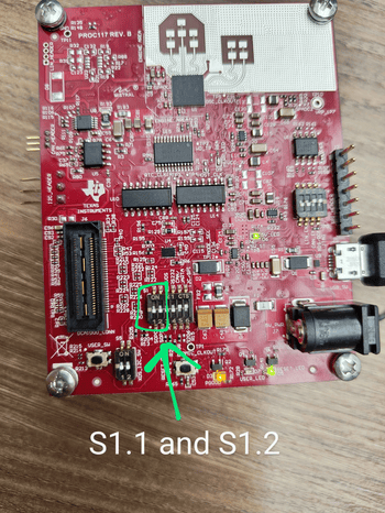
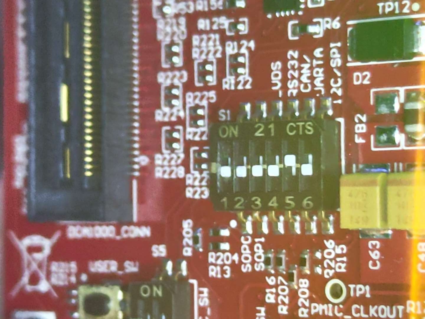
4. Switch the board to flashing mode by setting S1.1 to OFF, then reset the board.

5. Open UniFlash, select the application port, and press Load Image. App Image used for data collection is available here.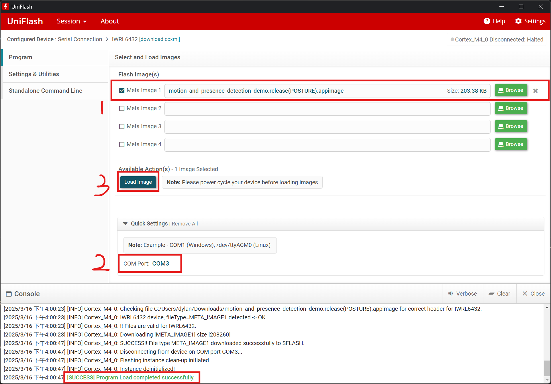
6. Switch the board back to running mode by setting S1.1 to ON, then reset the board.
7. Congratulations! You have successfully flashed the appimage to the board.

Training A Model

1. Setup

Before starting data collection, ensure the following steps are completed:

• Hardware Setup:
  • Position the mmWave radar board according to the predefined configuration (Check Data Collection Section).
  • Adjust the height, orientation, and distance from participants.
  • Verify sensor calibration.
  • Flash the appimage into the board by using UniFlash
• Software Setup:
  • Connect the radar board to the computer.
  • Flash the board with the provided firmware.
  • Ensure the correct Python environment is set up.

2. Data Collection Procedure

1. Connect the mmWave radar to your computer.
2. Run the TI-provided Python script to start data collection: python L6432_Parsing.py -p COM44 -c TrackingClassification_MidBw-POSE-115200
   • The parser is reading the data from the radar as per the TLV formats which are documented here and outputting a CSV file that is time coded in the name.

NoteBook Dependancies

Ensure you have Python installed on your system. You can check your Python version by running:

python --version

Python 3.7 or higher is recommended.

If you don’t have Python installed, download it from python.org and install it.

It is also recommended to use a virtual environment to avoid conflicts. We used separate anaconda environments for running the notebook and running the TVM compiler.

Installing the Packages

1. Install PyTorch

PyTorch installation depends on your operating system and whether you want to use CPU or GPU acceleration. Visit the official PyTorch website to get the exact command for your setup.

For CPU installation:

pip install torch torchvision torchaudio

2. Install Install Other Dependencies

pip install pandas scikit-learn torchmetrics matplotlib torchinfo onnx_tool

Verifying Installation

After installation, verify that the packages are installed correctly by running:

python -c "import torch, pandas, sklearn, torchmetrics, matplotlib, torchinfo, onnx_tool; print('All packages installed successfully!')"

If you see All packages installed successfully!, the installation is complete.

Additional Notes

If you face dependency issues, try updating pip first:

pip install --upgrade pip

If using Jupyter Notebook, install ipykernel to ensure compatibility:

pip install ipykernel

NoteBook Overview

1. Loads system parameters (CPU and/or GPU) that will be used for training
2. Loads the data from the datasets provided and compiles them into one dataframe for each classification
3. Extracts desirable features from the data, export the features for CCS testing later on, and turn these features into tensors for training
4. Defines the model architecture.
5. Trains the model with parameters at the top of the notebook
6. Exports the model to an ONNX file that can later be converted into C library.

How to use notebook (Pose Model Specific)

1. Save training data in the form of CSV’s the the dataset directory shown below. File names for each classification should match with the classification dictionary in the first module of the notebook (not caps sensitive).

2024-MMWAVERADARSENSORS
└── model
    ├── posture                                                        
    │   └── dataset
    |       └── classes
    |           ├── stood/    # Stood data CSV(s) go here
    |           ├── sat/      # Sat data CSV(s) go here
    |           ├── lying/    # Lying data CSV(s) go here
    |           ├── sitting/  # Sitting data CSV(s) go here
    |           └── falling/  # Falling data CSV(s) go here                                   

# Enumeration for each Category, \/\/\/\/\/ add new categories here along with data CSV's in a folder of same name 
class_data = {0: 'STOOD', 1: 'SAT', 2: 'LYING', 3: 'SITTING', 4: 'FALLING'}

1. Setup options for the notebook in the first module
   • VISUALSE (TRUE/FALSE): Whether to generate graphs of training data
   • WINDOW_SIZE (integer): Windows size of the frame data being used to training
   • WINDOW_CONCATENATE (TRUE/FALSE): Sort the windowed data or not
   • MIN_POINTS (integer): Number of points required for each frame of data from the radar board (will result in number of min and max height points = MIN_POINTS / 2)
   • EQUALISE_DATA_LENGTHS (TRUE/FALSE): Whether to make all datasets for each classifications equal in length
   • FILTER (TRUE/FALSE): Whether to filter the data collected (also requires filtering values)
   • NUM_EPOCHS (integer): Number of epochs of training to run
   • BATCH_SIZE (integer): Size of batches used when training the model
   • TEST_SIZE_PERCENTAGE (integer): Percentage (out of 100) of data collected to be not used for training but for testing the model instead
   • Learning Rate (float): Learning rate of the optimizer which determines the step size at each iteration while moving toward a minimum of a loss function
   • F1_SCORE_THRESH (float): Threshold for converting input into predicted labels for each sample
2. Run all of the modules of the notebook, the final module will generate the .onnx file containing the model

Compiling the Model

Setup TVM Environment

1. Verify python version

   which python3 
   - /usr/bin/python3
   python3 --version
   - Python 3.10.12
   

2. Install the wheel. Only works on Linux (We used Ubuntu 22.04). The wheel file is available here.

   pip uninstall ti-tvm -y
   pip install  ti_tvm-0.16.0-cp310-cp310-linux_x86_64.whl --force-reinstall
   

3. Verify installation

   tvmc -version
   - 0.16.0
   

4. Install the TI cross-compiler for the cortexM4

   wget https://dr-download.ti.com/software-development/ide-configuration-compiler-or-debugger/MD-ayxs93eZNN/2.1.2.LTS/ti_cgt_armllvm_2.1.2.LTS_linux-x64_installer.bin
   

   chmod +x ti_cgt_armllvm_2.1.2.LTS_linux-x64_installer.bin
   

   ./ti_cgt_armllvm_2.1.2.LTS_linux-x64_installer.bin
   

5. Following Ubuntu packages may be required before testing the compiler package

   sudo apt install libllvm14
   sudo apt install libncurses5
   tiarmar --version 
   -  TI LLVM version 14.0.6
   -  Optimized build.
   -  Default target: arm-ti-none-eabi
   -  Host CPU: haswell
   

6. Add below into ~/.profile for accessing compiler from the model folder

   PATH="$HOME/.local/ti-cgt-armllvm_2.1.2.LTS/bin::$PATH"
   

Compilation

1. Simply, set the options for the TVM compiler commandline tool.

   export TVMC_OPTIONS="--target-c-device=cortex-m4 --runtime=crt --executor=aot --executor-aot-interface-api=c --executor-aot-unpacked-api=1 --pass-config tir.disable_vectorize=1 --pass-config tir.usmp.algorithm=hill_climb --output-format=a"
   export TIARMCLANG_OPTIONS="-Os -mcpu=cortex-m4 -march=armv7e-m -mthumb -mfloat-abi=hard -mfpu=fpv4-sp-d16"
   

2. Then, run the command to compile the model.

   tvmc compile $TVMC_OPTIONS --verbose --target="c" ./my_Linear_model.onnx -o artifacts_M4F_soft_Linear/posture_model.a --cross-compiler="tiarmclang" --cross-compiler-options="$TIARMCLANG_OPTIONS"
   

3. Confirm devc.o, lib0.c, lib1.c, mod.a, and tvmgen_default.h are generated.

Using CCS

Importing the CCS projects

1. In the top toolbar click File -> Open Projects From File System
2. Click Directory and select CCS_Projects from the repository
3. Tick the projects you want to import
4. A restart of CCS may be required before running the projects if importing the projects for the first time

Running a CCS Project

1. Flash the empty appimage onto the board.
2. (First time only) Create a Target Configuration for the board
   • View -> Target Configurations
   • Right Click Window and select “New Target Configuration
   • Specify file name and check “Use shared location”
   • In the configuration editor window select Texas Instruments XDS110 USB Debug Probe and select IWRL6432 for board or device.
   • Press the “Save” button and optionally press “Test Connection” to verify configuration is functional.
3. Launch the configuration
   • Reset the board before connecting configuration
   • View -> Target Configurations
   • Right click target configuration and select “Launch Selected Configuration”
   • Right click Cortex_M4_0 core and select “connect target”
4. Run the project

   • Select Cortex_M4_0 so that it is highlighted and click the Load button in the toolbar

     

   • Press browse project and select the appropriate .out file generated from building a project (see below)

   • Select Cortex_M4_0 again and press the Run/Resume button

     

   • The program should start executing and generating console output

Test the Model

1. Copy data binaries containing formatted data generated by the notebook into the CSS project.
   • Notebook data binaries located in model -> posture -> dataset
   • Destination folder located in ccs_test_POSE -> dataSets
2. (First Time Only) Change dataset location variables in project
   • In project view open ccs_test_POSE -> pose.h

   • Change the variables with the path your project replaced

     

3. (IF MODEL HAS BEEN CHANGED) Copy Model files into the CCS project.
   • Generated model files located in model -> posture -> artifacts_M4F_soft_Linear
   • Copy posture_model.a and tvm_default.h into ccs_test_POSE -> model
   • Copy lib0.c and lib1.c into css_test_POSE -> model -> src
4. (IF THE FEATURES HAVE BEEN CHANGED) Change feature count variable in CCS
   • In project view open ccs_test_POSE -> pose.h

   • Change ML_TYPE3_FEATURE_COUNT to the appropriate number.

     

5. (IF THE CLASSIFICATIONS HAVE BEEN CHANGED) Change classification parameters in CCS
   • In project view open ccs_test_POSE -> pose.h
   • Change the variables containing the location of the dataset binaries (as seen above)

   • Change number of classes to appropriate number

     

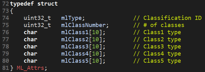
   • Change struct defining the model output structure to contain the correct number of classes

     

   • Open ccs_test_POSE -> pose.c

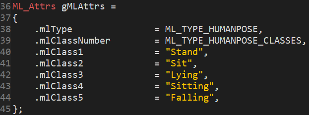
   • Change struct for containing the model output to contain the correct classes/class names

     

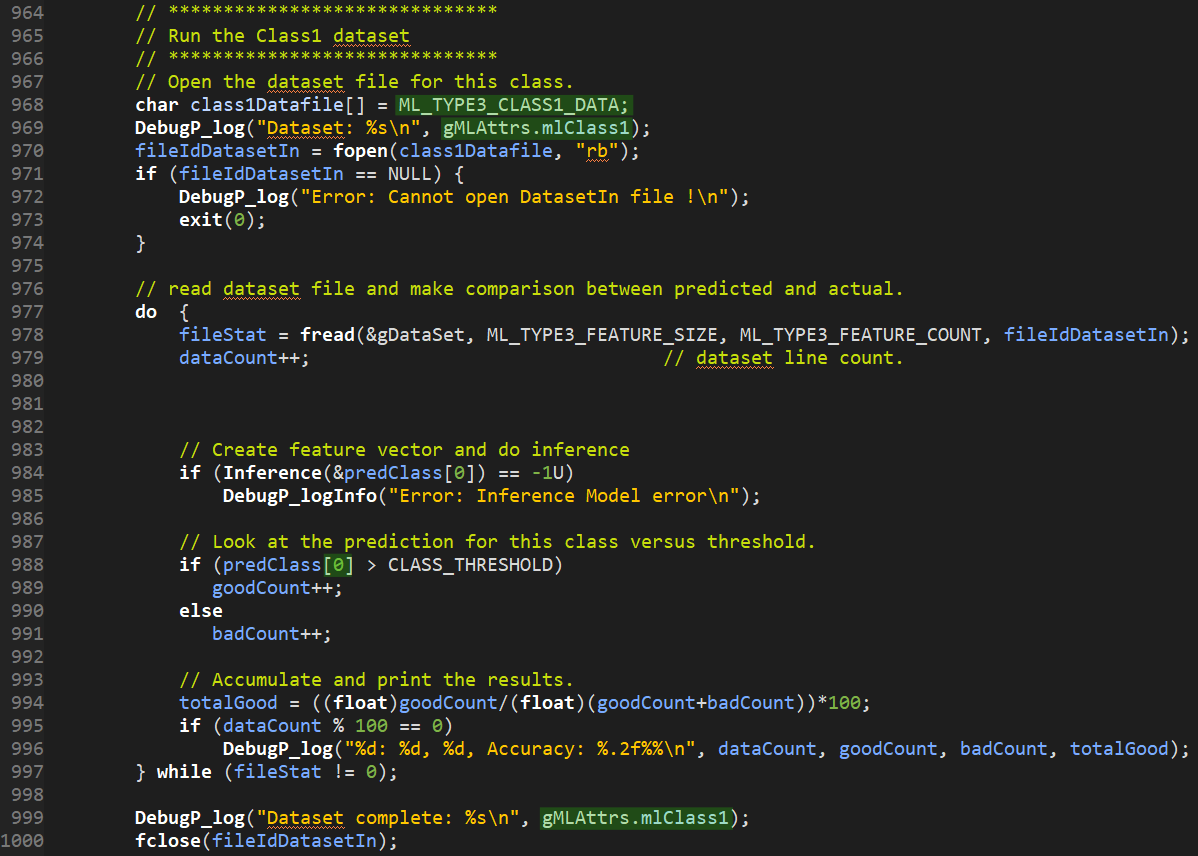
6. (IF THE CLASSIFICATIONS HAVE BEEN CHANGED) Change the code doing inference over datasets
   • In project view open ccs_test_POSE -> mmw_cli.c
   • Code running inference is located around line 950
   • Add/Remove procedures running inference on each class

   • Additional procedures can be copied from existing ones by changing variables highlighted below (Dataset Binary, Class Name, Class Number-1, Class Name)

     

7. Run the project to test the model

   • Build the project using the build button in the toolbar

     

   • Plug in the board via USB
   • Follow steps above to run the project
   • Click resume again once console output of memory configuarations is complete
   • Observe the results of the model test

Demo the Model

1. (IF MODEL HAS BEEN CHANGED) Copy Model files into the CCS project.
   • Generated model files located in model -> posture -> artifacts_M4F_soft_Linear
   • Copy posture_model.a and tvm_default.h into ccs_demo_POSE -> model
   • Copy lib0.c and lib1.c into css_test_POSE -> model -> src
2. (IF THE FEATURES HAVE BEEN CHANGED) Change feature count variable in CCS
   • In project view open ccs_demo_POSE -> pose.h

   • Change ML_TYPE3_FEATURE_COUNT to the appropriate number.

     

3. (IF THE FEATURES HAVE BEEN CHANGED) Change feature generation in CCS
   • In project view open ccs_demo_POSE -> motion_detect.c
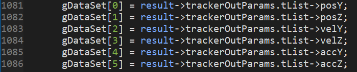
   • Track features are assigned around line 1080, point cloud features are assigned around 970.

   • Change variables assigned to gDataSet as required. Size of gDataSet is equal to feature count set above

     

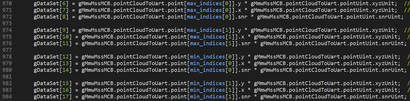
   • If the number of points being provided to the model per row has been changed also change the minimum count located in ccs_demo_POSE -> pose.h

     

4. (IF THE CLASSIFICATIONS HAVE BEEN CHANGED) Change classification parameters in CCS
   • In project view open ccs_demo_POSE -> pose.h

   • Change number of classes to appropriate number

     

   • Change struct defining the model output structure to contain the correct number of classes

     

   • Open ccs_demo_POSE -> pose.c

   • Change struct for containing the model output to contain the correct classes/class names
5. Run the project to demo the model

   • Build the project using the build button in the toolbar

     

   • Plug in the board via USB
   • Follow steps above to run the project
   • Click resume again once console output of memory configuarations is complete
   • At this point the board is communicating results over UART. They can be viewed using the visualiser program provided

Visualiser

Once the board is running a model and is sending results over UART. The visualiser can be used to see the classification and point cloud data.

1. Navigate to the directory containing the visualiser program. visualiser\
2. Run python main.py.

3. If there is a COM port error the default COM port is incorrect. This is fine and the program should load anyway.

   

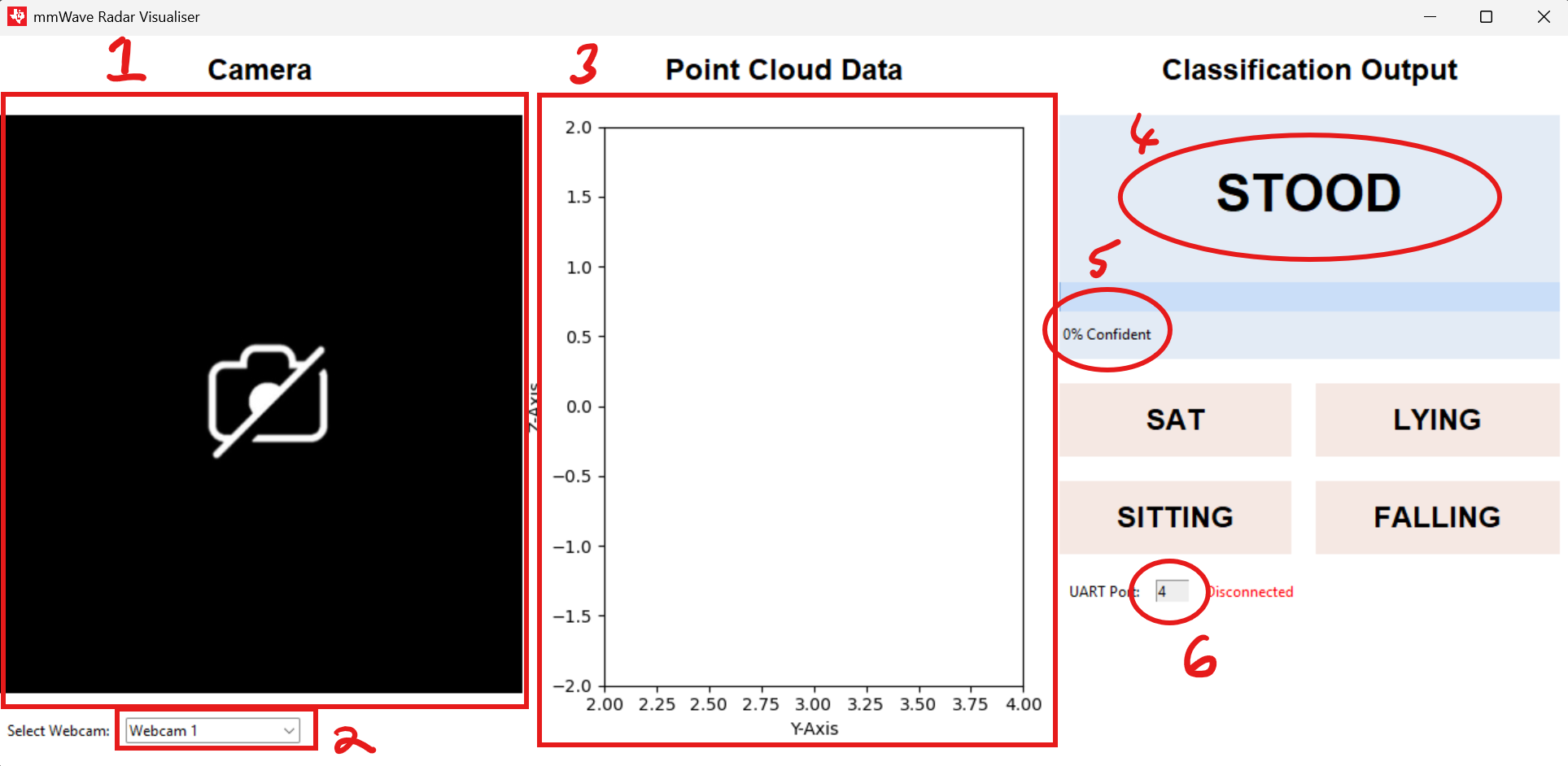
Visualiser Overview

1. Camera View
2. Camera Select
3. Point Cloud data View
4. Classification Result
5. Confidence Level
6. UART Port Select

Changing COM port

1. Enter the desired COM port number
2. Press enter
3. Check for “Connected” text

Changing Camera

1. Select camera select dropdown
2. Choose desired camera

Data Viewer

This tool can be used to go through any data collected using the data collection script. Opening the csv file created by the python script will display the data in an animated way, the user can pause the visualisation whenever they like.

1. Navigate to the directory containing the CSV data viewer program visualiser\graph\.
2. Run python csv_ui.py.
3. There is an example csv file in the same directory example.csv that can be used to test the software.

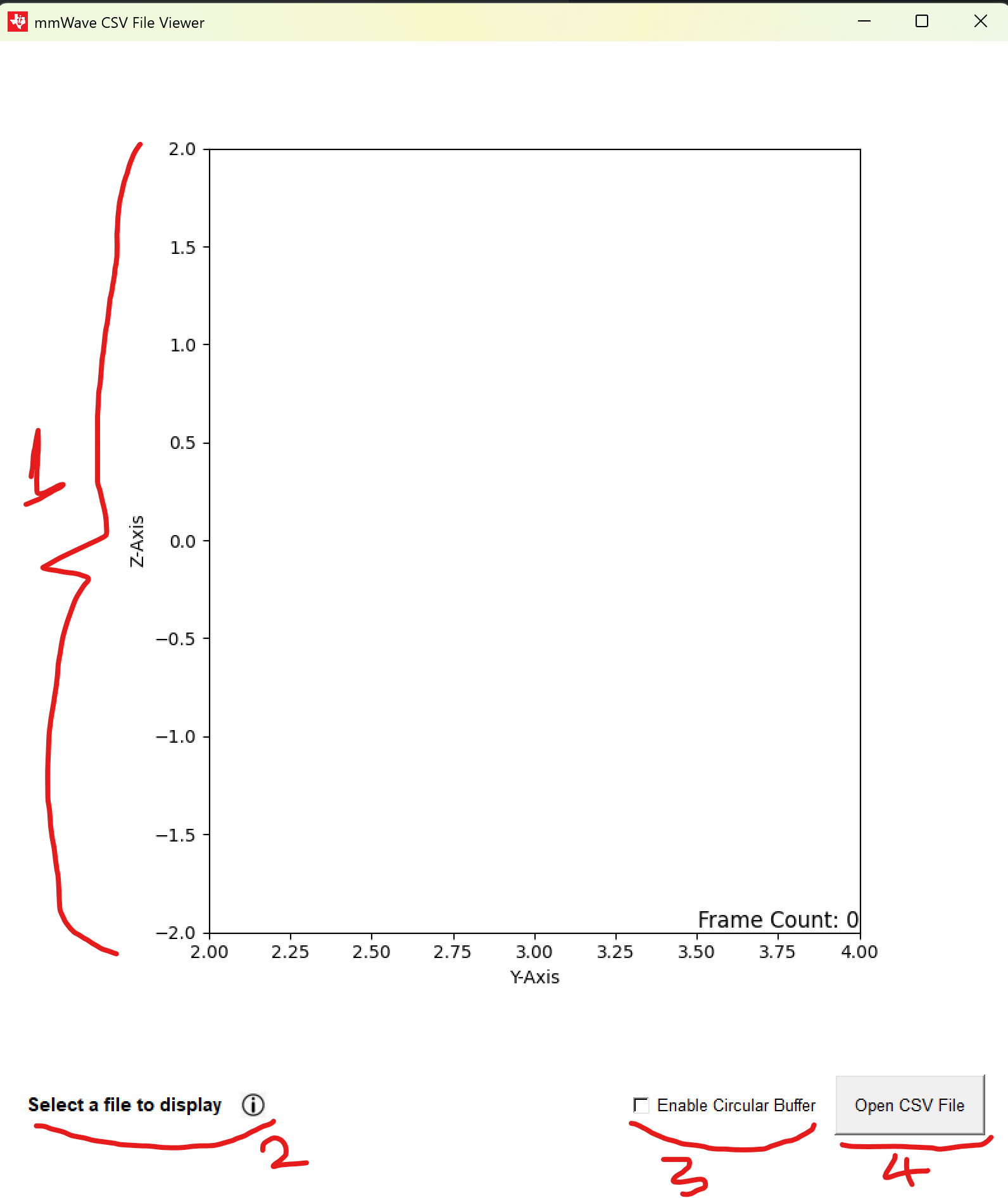
Data Viewer Overview

1. Point Cloud Data View
2. Info Icon
3. Circular Buffer Mode Checkbox
4. File Select

Info Icon

Hovering over the info icon will give the user helpful instructions, the text next to the icon informs the user on whether the visualisation is paused or not when a csv file is being viewed. The user can press space to pause/resume the recording whenever they like.

Circular Buffer

The machine learning model has a window size of 5, meaning that it looks at the 5 most recent frames before determining the posture. By enabling this checkbox the user can view the latest 5 frames, disabling this will only show the current frame.